Overview: 2x2 R-commands
In this section we describe the basic commands for 2x2 inference. For
this purpose, and without loss of generality, we use the running example
from the book portrayed in Table 2.3 (page 31). This example uses the
proportion of the voting age population who are black
(),
the proportion turning out to vote
(),
and the number of voting age people
()
in each precinct
()
to infer the fraction of blacks who vote
()
and the proportion of whites who vote
(),
also in each precinct. (For an extended example of ei,
refer to the user’s guide below.) An example of a sequence of these
commands are as follows:
library(ei)
data(matproii)
formula <- t ~ x
dbuf <- ei(formula = formula, total = "n", data = matproii)
summary(dbuf)
plot_tomog(dbuf)
plot_xt(dbuf)
In most applications, plot and eiread would
likely be run multiple times with different options chosen, and other
commands would be included with these five to read in the data
(t, x, and n).
ei: To run the main procedure
Use the format,
dbuf = ei(formula, total = "n", data = data), which takes
three
vectors as inputs: t (e.g. the fraction of the voting age
population turning out to vote); x (e.g. the fraction of
the voting age population who are black); and n (e.g. the
total number of people in the voting age population). The output of this
procedure is the list dbuf (i.e. an output object of class
list called a “data buffer”). The data buffer includes the maximium
likelihood estimates and simulated quantities of interest from the
ei procedure. After running ei, it is a good
idea to save dbuf for further analysis. The output data
buffer from ei includes a large variety of different
results useful for understanding the results of the analysis. A minimal
set of nonrepetitive information is stored in this list (or data
buffer), and a large variety of other information can be easily computed
from it. Fortunately, you do not need to know whether the information
you request is stored or computed as both are treated the same.
To extract information from the data buffer, three procedures are available:
summary: To obtain a general summary of district-level
information
summary(dbuf) will produce aggregate information about
the ei results. summary will produce a summary
of both the maximum likelihood estimates and simulated quantities of
interest. It also includes information on the values specified for the
prior.
plot: To graph relevant information
For graphics, use plot_**(dbuf);, where
dbuf is the ei.object that is the output of ei
or ei.sim, and ** completes a function for
ready-made graphs. For example, plot_tomog(dbuf) will plot
a tomography graph, and plot_xt(dbuf) will display a
scattercross graph. Any number of graphs can be selected in plot for
output.
Some of the plots can be produced after estimating the maximum
likelihood estimates using ei, but before simulating
quantities of interest. These initial plots can be useful in determining
which priors to include, and the user can opt to choose not to simulate
quantities of interest by selecting the option
simulate = FALSE. However, for some plots,
plot will need the simulated quantities of interest, and
therefore can only be plotted when simulate is set to the default,
TRUE.
eiread: To obtain relevant information and numerical
results
For numerical information, use
v <- eiread(dbuf, "name"), where v is the
item extracted, dbuf is the data buffer output from
ei, and name can be any of a list of output possibilities.
For example, eiread(dbuf, "betab") will give a vector of
point estimates of
,
eiread(dbuf, "ci80w") will give 80% confidence intervals
for
.
Any number of items can be selected for output. For example,
eiread(dbuf, "betab", "ci80b") will produce a list of the
point estimates and 80% confidence intervals for $ _i^b$.
User’s Guide: An Example
We now show how to use ei through a simple example. We
use data on voter registration and racial background of people from 268
counties in four Southern U.S. States: Florida, Louisiana, and South
Carolina. These are the same data used in Chapter 10. The data include
the total voting age population in each county (n), the
proportion of the population in each county who are black
(x), and the proportion of the population in each county
who are registered to vote (t). The proportion of whites
registered can be computed by (1-x). You can load the data
into R using the command
library(ei)
#> Loading required package: eiPack
#>
#> Attaching package: 'ei'
#> The following object is masked from 'package:stats':
#>
#>     filter
data(matproii)
The statistical goal is to estimate the fraction of blacks registered
()
and the fraction of whites registered
()
in each county. These quantities of interest are generally unknown.
However, ei also includes an option that allows the user to
assess the reliability of the ei algorithm when the true
quantities of interest are known. To illustrate the use of this “truth”
option, the data also include the true fractions of registered blacks ()
and the true fraction of registered whites (tw).
The Basic EI Algorithm
To begin, we perform ecological inference by calling the function
ei. ei first computes and maximizes a
likelihood distribution based on the inputed data, then estimates the
county-level quantities of interest based on the possible values, or
``bounds”, for each county and the overall likelihood distribution.
To run this algorithm, at a minimum we need to have three vectors.
Two vectors, t and x, contain the aggregate
known information about the counties of interest. In this example,
t is the proportion of voters registered in each county,
and x is the proportion of blacks in each county. These two
vectors contain aggregate information, since we are interested in the
proportion of voters in each country who are black. The last vector we
need is n, the number of people of interest in each county.
In this example, n is the number of people of voting
age.
We proceed by performing ecological inference without covariates on the data:
formula <- t ~ x
dbuf <- ei(formula = formula, total = "n", data = matproii)
#> ℹ Running 2x2 ei
#> ℹ Maximizing likelihood for `erho` = 0.5.
#> ℹ Running 2x2 ei✔ Running 2x2 ei [3ms]
#>
#> ⠙ Beginning importance sampling.
#> ✔ Beginning importance sampling. [165ms]
To include a covariate on simply specify a covariate vector for the option , or a string that refers to the name of the covariate in the dataset. Similarly, to include a covariate on , specify a covariate vector for for the option , or a string that refers to the name of the covariate in the dataset.
Next, we use summary(dbuf) to obtain general information
about the estimation.
summary(dbuf)
#>
#> ── Summary ─────────────────────────────────────────────────────────────────────
#>
#> ── Erho ──
#>
#> 0.5
#>
#> ── Esigma ──
#>
#> 0.5
#>
#> ── Ebeta ──
#>
#> 0.5
#>
#> ── N ──
#>
#> 268
#>
#> ── Resamp ──
#>
#> 19
#>
#> ── Maximum likelihood results in scale of estimation (and se's) ──
#>
#>        Bb0       Bw0       sigB       sigW       rho Zb0 Zw0
#>  1.2671900 1.9349556 -1.1149542 -1.3270775 1.6053564   0   0
#>  0.2846636 0.2826169  0.2140042  0.1646036 0.3145764   0   0
#>
#> ── Untruncated psi's ──
#>
#>         BB       BW        SB        SW       RHO
#>  0.9905045 1.152859 0.3368288 0.2760415 0.9179783
#>
#> ── Truncated psi's (ultimate scale) ──
#>
#>         BB        BW       SB        SW       RHO
#>  0.6199244 0.8259608 0.198239 0.1423288 0.7695587
#>
#> ── Aggregate Bounds ──
#>
#>           betab     betaw
#> lower 0.2125903 0.7025925
#> upper 0.9754242 0.9200036
#>
#> ── Estimates of Aggregate Quantities of Interest ──
#>
#>         mean          sd
#> Bb 0.5711949 0.024469142
#> Bw 0.8177997 0.006973817
#>
#> ── Precision ──
#>
#> 4
#>
The summary function provides basic information about
the ecological inference estimation, the maximum likelihood estimates on
three scales, and an overall summary of the quantities of interest.
First, it reports the values of the priors used in ecological inference
(Erho, Esigma, Ebeta). It also reports the number of
counties in the dataset (N), as well as the number of
importance sampling iterations required to produce estimates of the
quantities of interest (resamp).
summary also produces information both about the maximum
likelihood estimates and the quantities of interest. First, it provides
the maximum likelihood estimates in the scale of estimation. Next, it
provides the values of the MLEs when they are transformed into an
untruncated bivariate normal distribution. These estimates provide
information about the location of the highest density of estimates for
the proportion of blacks who are registered to vote and the proportion
of whites who are registered to vote. Last, it provides the values of
the MLEs on the ultimate truncated bivariate normal scale. These
estimates are an unweighted average of the fraction of blacks and whites
registered to vote over all the counties in the sample. In this example,
the ei algorithm predicts that the unweighted average of
the proportion of blacks registered to vote across counties is 0.57 and
the unweighted average of the proportion of whites registered to vote is
0.82.
Finally, summary produces information on aggregrate
quantities of interest. The aggregate bounds are the mean of the bounds
on the proportions of black and white voters, weighted by the population
in each county. The aggregate quantities of interest are the weighted
mean of the proportion of registered blacks and the proportion of
registered whites in each county. In this example the weighted average
proportion of blacks who are registered is 0.57, and the weighted
average proportion of whites who are registered is 0.82.
Extracting Quantities of Interest
eiread extracts quantities of interest in a list format
from the object dbuf. For example,
bb.out <- eiread(dbuf, "betab", "sbetab")extracts the point estimates and estimated standard deviations for
,
the estimates of the proportion of registered blacks in each county. The
user can then use bb.out$betab to obtain a vector of the
point estimates for
,
and bb.out$sbetab to obtain a vector of the standard
devations for
.
eiread() takes any number of arguments to extract any
number of quantities of interest from the data buffer.
?eiread can be used to find a list of quantities of
interest that are available in ei. Among the most useful
arguments are "betab" and "betaw", which
report the point estimates; "sbetab" and
"sbetaw", which report the standard deviations of the point
estimates; and "CI80b and "CI80w", which
report the confidence intervals of the point estimates.
Plotting in EI
Plotting ei output is extremely useful for understanding
the results of the ecological inference algorithm and diagnosing
problems with estimation. First, we graph a tomography plot of the data
(Figure 1).
plot_tomog(dbuf)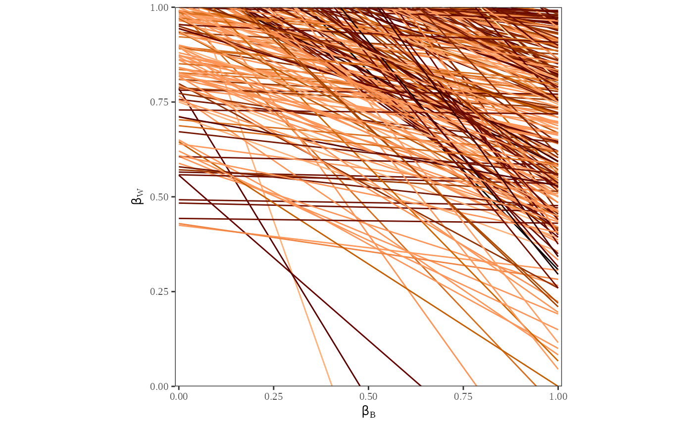
Tomography Plot with ML Contours:
plot_tomog(dbuf, options = list(contour_ML = TRUE))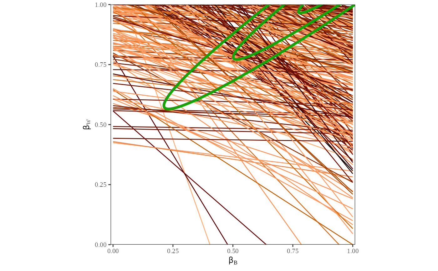
Tomography Plots with Point Estimates
plot_tomog(dbuf, options = list(points = TRUE))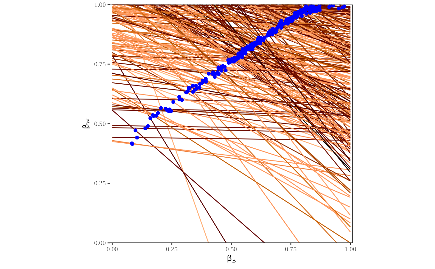
Tomography Plots with Confidence Intervals
plot_tomog(dbuf, options = list(CI = 0.95))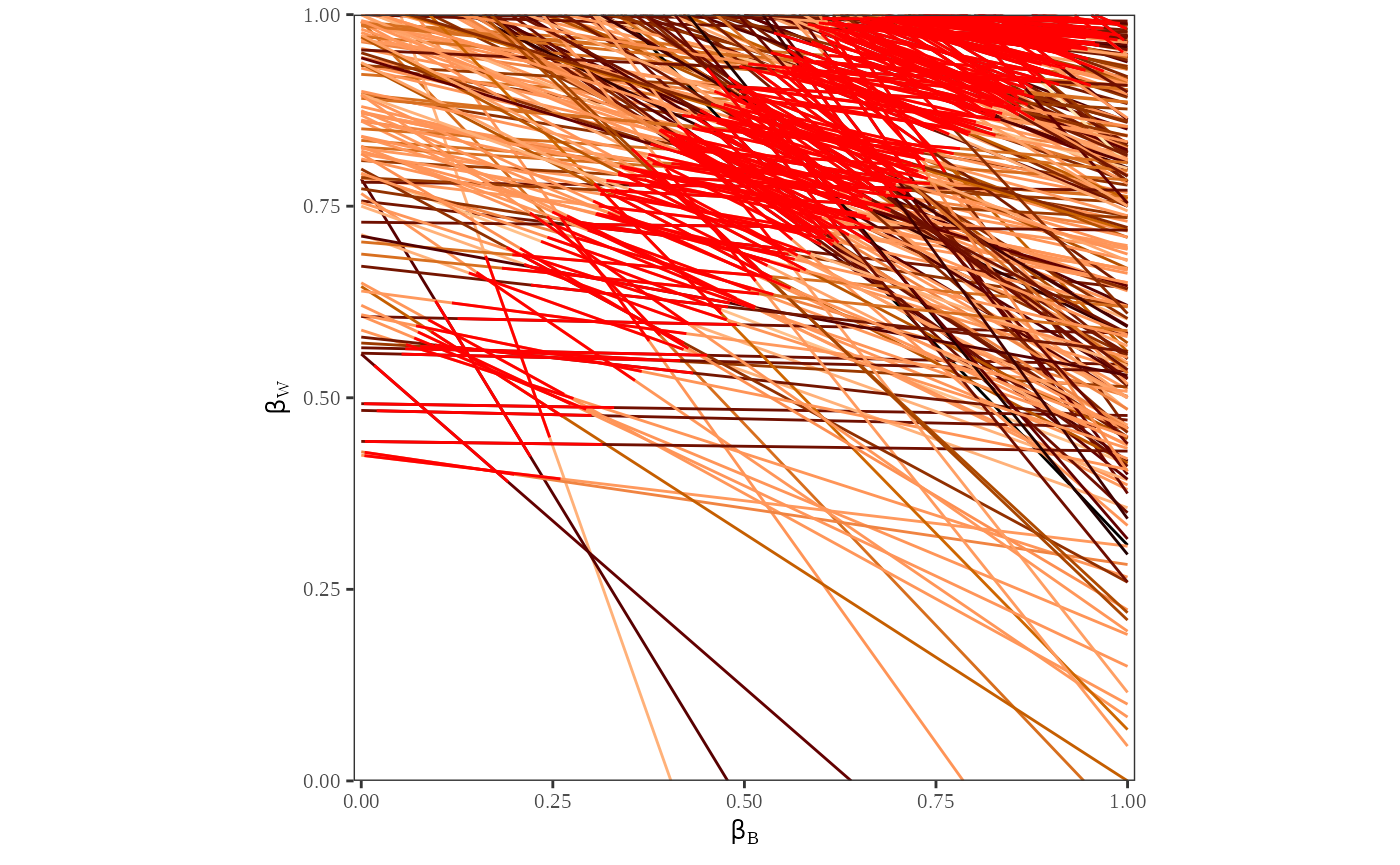
Each line on the map represents the possible values for and for one county. The contour lines identify the portion of the lines that have the highest probability of containing the true estimates of and . These contour lines provide information about the overall pattern of registration. Note that the area with highest probability is in the upper right-hand corner, where the proportion of whites registered is between and and the proportion of blacks registered is between and . Further, we see that the lines are clustered in the upper half of the figure, indicating that the possible values of will have a lower variance than the possible values of .
Figure 2 is a double plot of the point estimates and their confidence intervals. To compute this, we call plot to generate two graphs: a tomography plot with the point estimates generated from the algorithm, and a tomography plot with 80% confidence intervals on the point estimate.
plot_tomog(dbuf, options = list(points = TRUE, CI = 0.95))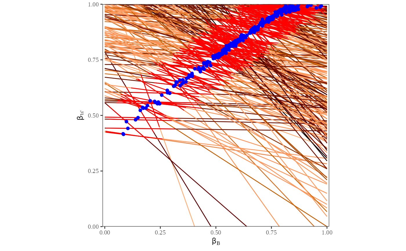
This plot is useful to visualize the estimates and confidence intervals for each county. We can see that the point estimates and confidence intervals are clustered in the same area as the contours from the previous plot. Further, the point estimates and confidence intervals only fall on the lines that indicate the possible values of and .
Figure 3 shows plots that indicate the distribution of and . To produce these plots, run:
plot_density(dbuf, options = list(parameter = "betab"))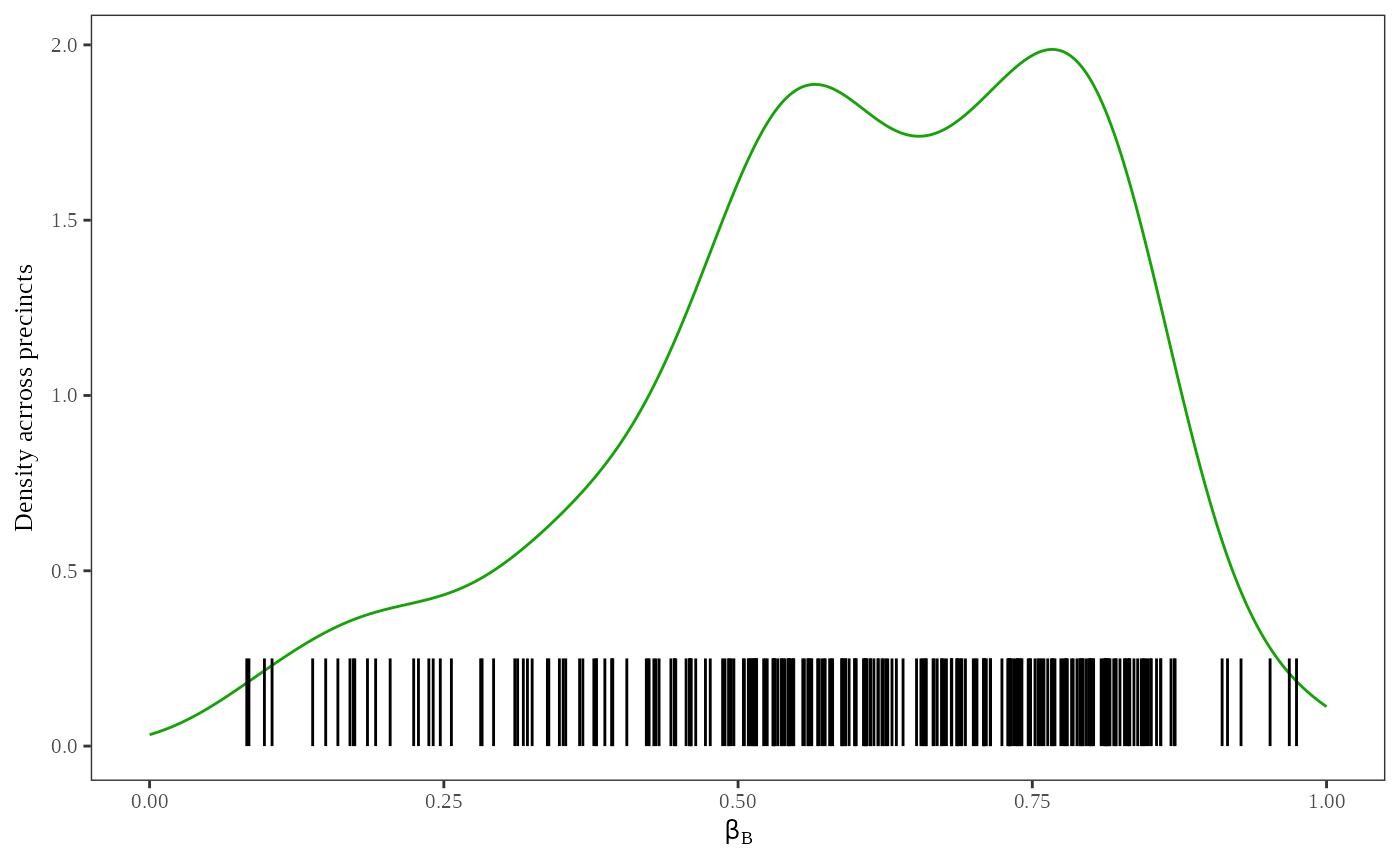
plot_density(dbuf, options = list(parameter = "betaw"))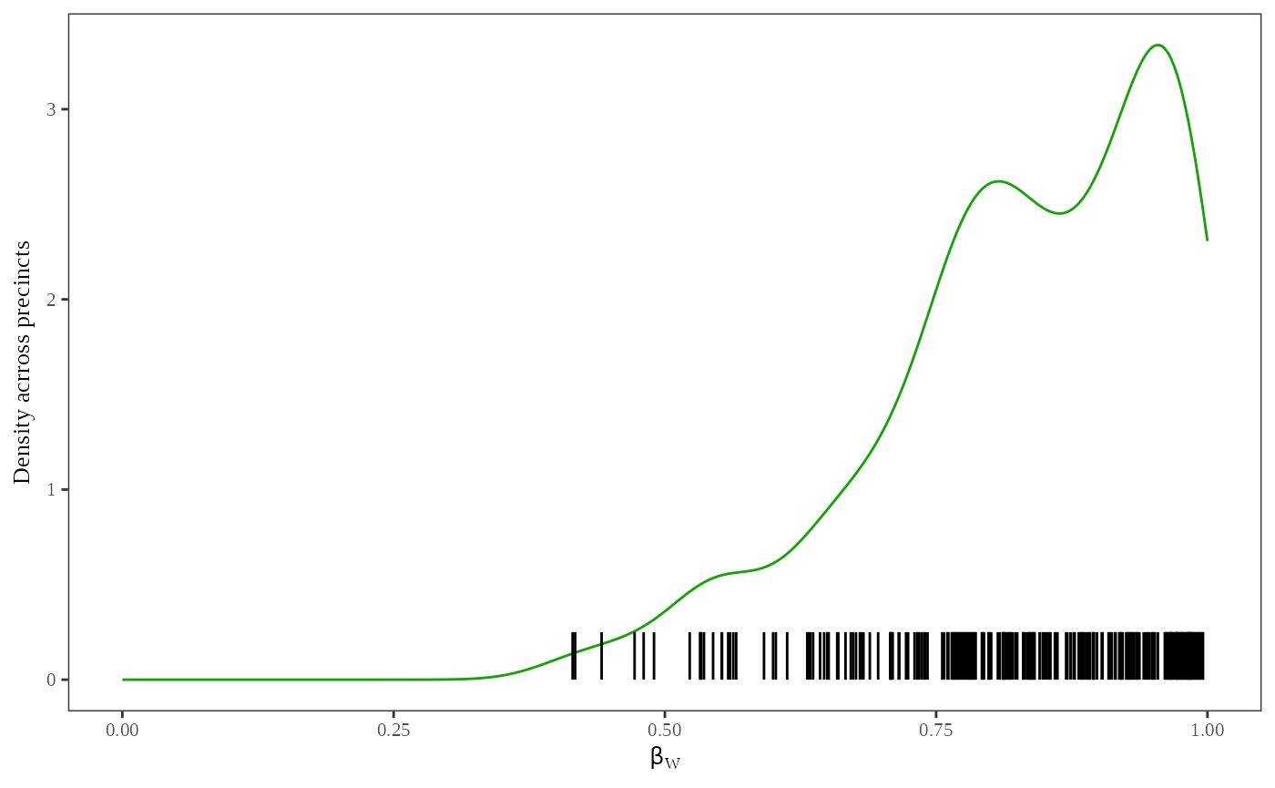
Density plots are useful to visualize the location and uncertainty of the point estimates. The green line represents the density of the simulated point estimates, and the black tick marks are a rug plot of the point estimates,s and . You can see that the variance of the point estimates from is much higher than the variance of point estimates from .
Figure 4 portrays the results of the ei algorithm by
plotting the proportion of blacks in each country by the proportion of
registered voters in each county. To produce this plot, use:
plot_xt(dbuf)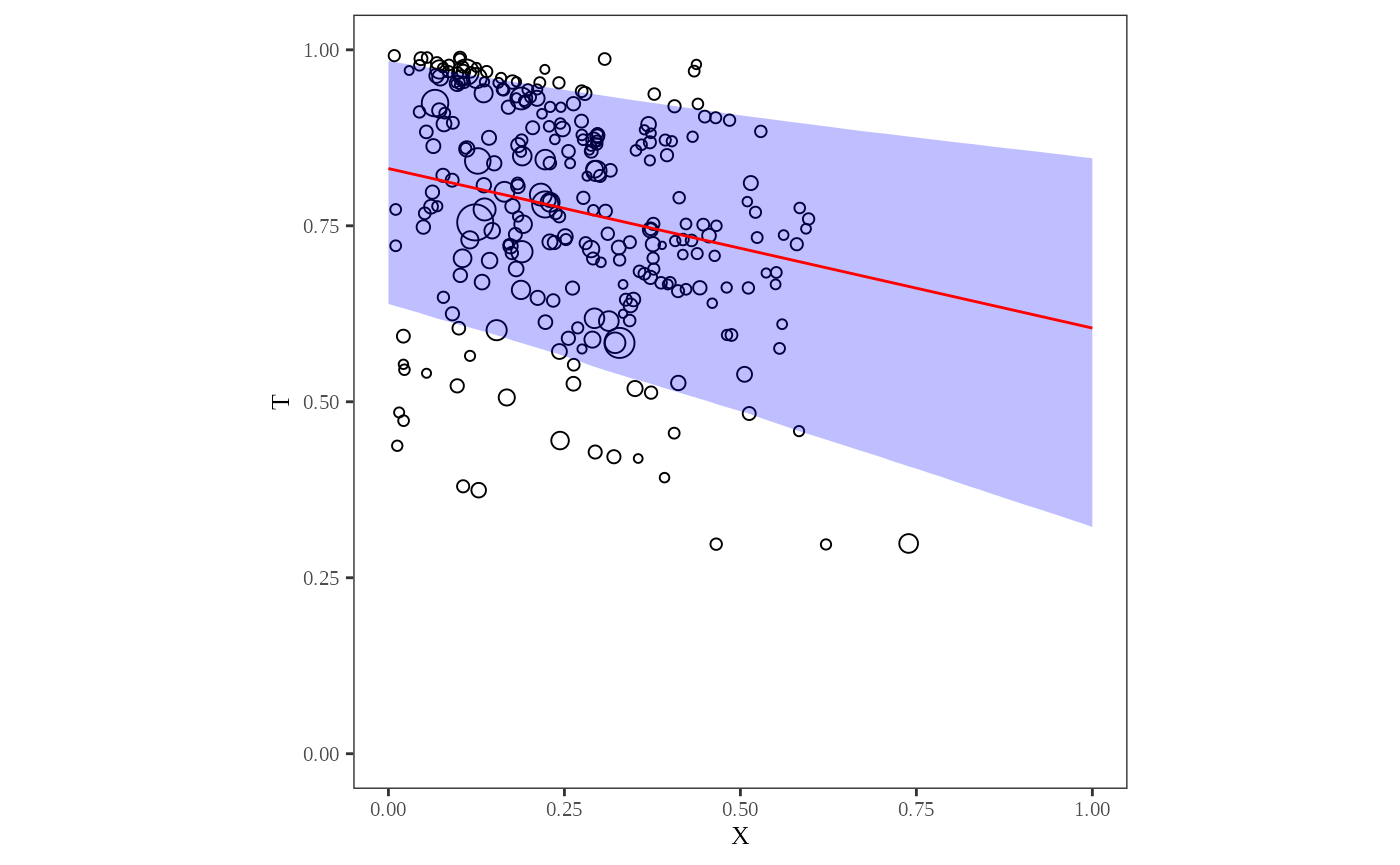
The circles around each of the points in this plot are proportional to the population of each county. The graph represents the likelihood estimates by plotting the expected number of registered voters given the proportion of blacks in each county, represented by the yellow line. The red lines in the plot are the 80% confidence interval around the regression line. The higher uncertainty in the estimates of black registration can be seen by the absence of points on the right hand side of the graph and the larger confidence interval on the right hand side of the graph, where the proportion of blacks in the county is relatively large.
Finally, if we have data on the true proportions of registered blacks
and registered whites in each county, as we do in this dataset, we can
use plots in ei to assess how well the algorithm works on
the given data. To do this, rerun the ei algorithm, adding
the truth vectors, and tw as the truth argument.
truth <- cbind(matproii$tb, matproii$tw)
formula <- t ~ x
dbuf_truth <- ei(formula = formula, total = "n", data = matproii, truth = truth)
#> ℹ Running 2x2 ei
#> ℹ Maximizing likelihood for `erho` = 0.5.
#> ℹ Running 2x2 ei✔ Running 2x2 ei [1ms]
#>
#> ⠙ Beginning importance sampling.
#> ✔ Beginning importance sampling. [191ms]
Then use plot to compare the estimates of the ei
algorithm to the true proportions of white and black registered voters
in each county.
# Comparing Estimates to the Truth at the County Level
plot_truth(dbuf_truth)
#> Warning: Using `size` aesthetic for lines was deprecated in ggplot2 3.4.0.
#> ℹ Please use `linewidth` instead.
#> ℹ The deprecated feature was likely used in the ei package.
#>   Please report the issue at <https://github.com/iqss-research/ei/issues>.
#> This warning is displayed once per session.
#> Call `lifecycle::last_lifecycle_warnings()` to see where this warning was
#> generated.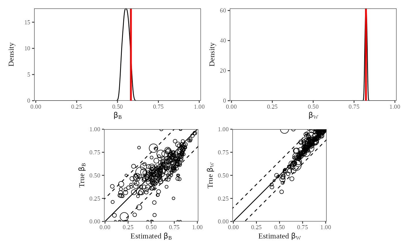
The “truth” plot (Figure 5) has four components. The top two figures have the posterior densities of the aggregate quantities of interest and . These densities tell us in what range the algorithm predicts that the point estimates lie. For example, the density of is wider than the density of , indicating that our estimates of lie in a smaller range than than our estimates of . The true aggregate values, computed from the data we inputed, are indicated by the vertical bars. The fact that the true and are within the densities we computed confirms that the model is did a good job at predicting the true proportions of registered white and black voters.
The bottom two figures in Figure 5 plot the estimated values of
and
against the true values. The size of each of the circles plotted is
proportional to the number of blacks in the county in the first graph
and the number of whites in each county in the second graph. If the
estimated values were exactly equal to the true values, all of the
points would be on the
line. Because the points fall quite close to the
and do not deviate from the line in a systematic way, we can see that
the ei algorithm predicts the point estimates quite
well.
References
Gary King, A Solution to the Ecological Inference Problem: Reconstructing Individual Behaviour from Aggregate Data, Princeton University Press (1997).
Gary King and Langche Zeng, “The Dangers of Extreme Counterfactuals.” Political Analysis, 14:2, pp 131-159, 2006.
Lau et al, “eiPack: Ecological Inference and Higher-Dimension Dtaa Management.” http://www.olivialau.org/software.
Rosen et al, “Bayesian and Frequentist Inference for Ecological Inference: The RxC Case.” Statistica Neerlandica, 55:2, pp 134-156, 2001.
Useful documentation also avalaible at http://gking.harvard.Edu.
For R language see http://www.r-project.org.
Venables, W.N.,and Ripley, B.D., Statistics and Computing, Springer (2002).